What’s New in SOLIDWORKS 2019: Simulation, Flow, & Plastics

Welcome, to our What’s New in SOLIDWORKS 2019 on Simulation, Flow, and Plastics. My name is Damon Tordini, I’m one of the project managers here at Hawk Ridge Systems, and along with me as well is Silvio Perez. He is also one of our project managers, and both of us focus on Hawk Ridge Systems simulation product suite, including SOLIDWORKS Simulation. In this webinar, we’ll review new features in SOLIDWORKS 2019 Simulation, Plastics, and Flow Simulation, specifically their topology optimization and thermal analysis enhancements.

Video Transcript

Introduction

We’re going to be taking you through a presentation over the next 45 minutes or so about the new enhancements in SOLIDWORKS 2019 that focus on these three add-ins for SOLIDWORKS and what new capabilities that they are gonna provide you guys when everyone upgrades to 2019 in terms of design validation and analysis. We’re going to start off by covering some of the enhancements for SOLIDWORKS Flow Simulation, which of course is our CFD tool, if you’re not familiar, uh, for simulating all the fluid flow and heat transfer problems that you might have on your SOLIDWORKS designs.

And then we’ll proceed to look at the enhancements for SOLIDWORKS Plastics, which is our injection molding simulation tool, it’s for predicting the plastic injection molding process, the manufacturing process, to see what the quality and the production speed of your plastic parts is. Then, I’ll be passing it over to Silvio, who’ll wrap up the presentation by looking at SOLIDWORKS Simulation and some of the FEA structural capabilities that have been added for 2019.

SOLIDWORKS Flow Simulation Enhancements

To start off with SOLIDWORKS Flow Simulation, which is again a CFD analysis tool built inside SOLIDWORKS. It is a wide-ranging tool that has a lot of capabilities but one of the most common uses for SOLIDWORKS Flow Simulation, especially among our customers here at Hawk Ridge Systems is to evaluate heat transfer and electronics cooling. And so there is a really cool enhancement for 2019 that I’m gonna show you that gives you a new type of result plot, which is sort of a graphical diagram that explains how the heat is being transferred around between different components in your assembly.

That will allow you to see the visual results on the model but through this new result graph, that’s kind of schematic. It’ll let you see which components are really contributing the most heat and what’s causing the other components to maybe heat up more than you expected. I’ll be showing you that in a second here. In conjunction with that, if you are then gonna go look at some surface results or maybe a cut plot which is kind of like a section plane of your results. You’ll be able to see surface parameters on that section plane as well now. For example, if you wanna know what the volume or mass flow rate is, you won’t have to go create a special kind of goal or measurement plane or anything like that in advance. You’ll be able to get that kind of feedback in real time when you’re looking at your cut plot results.

Let’s take a look at a couple of those things first, and while we’re going into SOLIDWORKS I will also show you briefly that there’s an enhancement to the custom visualization parameters. These are special user-defined result plots that you can create. For example, if you wanted to see velocity but only in the Y direction, you can create that and you can put in simple mathematical formulas to combine those things.

For example, in one velocity in one direction plus velocity in another. We’ve added some capabilities in 2019, where you can now also have, uh, mathematical expressions and logical expressions in those results too. So if statements or-or and statements. So let’s jump into SOLIDWORKS and I’ll show you a couple of those things. So this is all over 2019. Again, the user interface is gonna to be very familiar for the rest of you that have already used SOLIDWORKS 2018 or other recent releases.

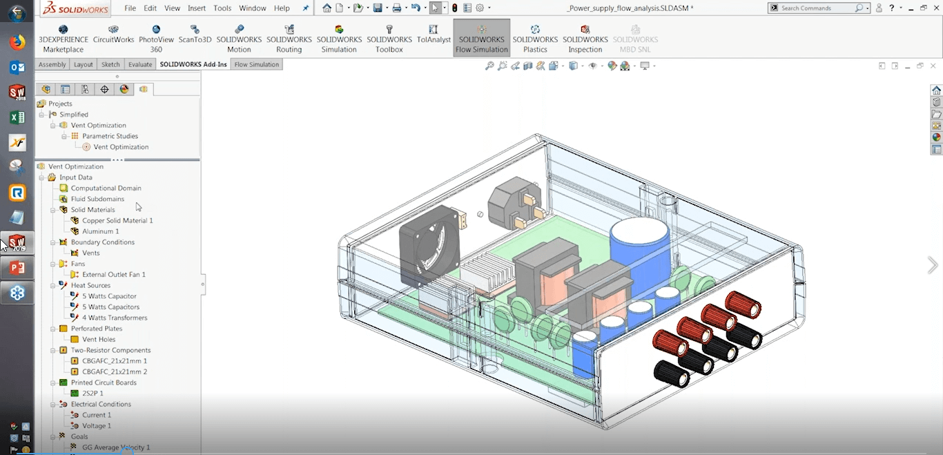
I can go ahead and turn on the flow simulation add-in for SOLIDWORKS just by clicking the button on the command manager there. And so this is a kind of a simplified power supply model that I’ve got. We’ve actually had this example for quite a while, but let’s see if we can teach it some new tricks in 2019. And so one of the things I want to show you are, let’s say, I’m running a thermal analysis on an assembly like this and I’ve got several different heat sources in this assembly.

For example, I’ve got also like five watts of heat from this large capacitor, maybe four watts on these transformers, and I’ve also got what we call the two-resistor components defined over here for these chips. This is a special input condition in the electronics cooling module for flow simulation that lets you put in the data you would get on the spec sheet for that chip.

And so I’ve got all of these heat generating components in my simulation. And of course, I’ve always been able to run my analysis and then load up my results and get things like the temperatures of the chips, or for example, a graphical plot of temperatures on the actual components. But if you wanted to find out what each of these components is sort of contributing to the other, how much heat is being sent between them, it was kind of hard to do just, you know, looking at these kind of visual surface plots, trying to do math in your head, or on paper when you went and looked at your regeneration results. So now there’s a special new result plot, a new type of schematic plot that will let you see that. And if you go to your flow simulation results, you’ll see there’s something called flux plot at the bottom of the list now.

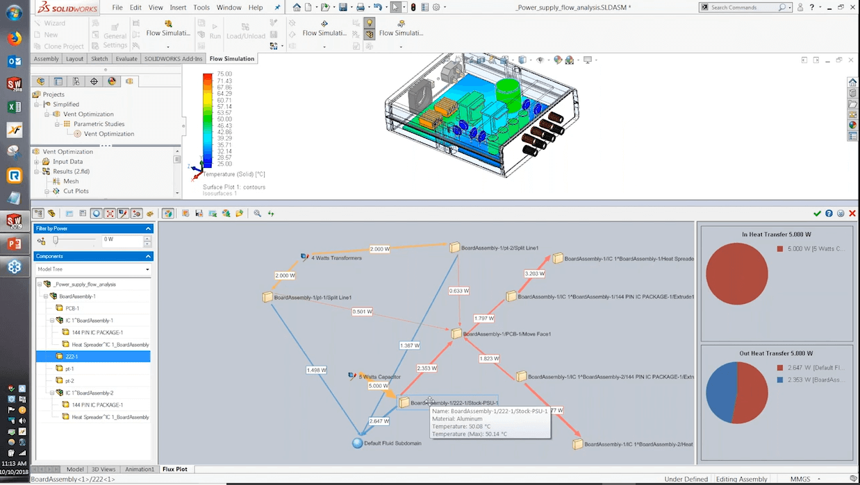
And so all I have to do for this flux plot is I can go and select the components that I wanna be included, like, for example, these transformers, and maybe the chips underneath the heatsink and maybe this capacitor over here. You can even select use all components if you wanted a really big, complex chart. And if you click okay, what you will see is this diagram that gets created for you, which you can zoom in on.

And it has a list of all of the different components that I’ve selected where it shows not only the heat source that is going into that component that I have defined in the project, but it also shows how much heat is being transferred from that component to the other. So for example, here, you can see I’ve got this component which is the transformer. When I click on it, it’s highlighting up there in the graphics area. And that’s sending about half of the watts over here to the PCB.

Or you can see here I’ve got this chip. This is the first integrated circuit and according to this, it is receiving a certain amount of heat from that component as well. You can see through the arrows there. And the same thing with these components down here. You can rearrange this and of course, take screenshots of or save the images directly, if you wanna present that. For example, a board layout designer who’s trying to decide, you know, maybe whether the components should be moved and which components are contributing to each other.

And you can also see a pie chart, you pop this up on the screen here. And that will show you, for each of these components. For example, how much heat is going in, how much heat is going out, and the proportions of them are. So again, all of these steps can be saved to image files or just screen captured. And it’s a more mathematical way to view what the contributions are from each of these components, um, to the temperatures of the system.

Cut Plot

Now, another popular way to visualize results besides just the surface plot is something called a cut plot. Some of you may have used that before. A cut plot, of course, is where you can take a section in your simulation and plot the results on it. Like for example velocity, you can see your velocity here. And so this is something that’s always been in flow simulation, but if I wanted to view the properties of this cut plot as I drag it around through the model for example, or maybe what’s the volume flow rate, or the average velocity, or the average temperature, or any other of the parameters on that plane, there wasn’t really an easy way to do it. You would have had to go in there and model an actual surface, and then measure those properties on that physical boundary.

Well, now, in 2019, if you want to use the surface parameters result in feature to measure all of those things, we can go into that parameter. And rather than selecting a face, which is what we used to have to do, we now have this new option at the end here called cut plot. And I can select from the drop-down menu which of the cut plots I’ve created in my results I wanna measure from. So for example, this plot here is cut plot two, so I can select that in the drop down.

And now if I hit show, I get all the parameters, like I normally do, down in my table view at the bottom. But I also can see the parameters displayed here on the screen in my graphics area, and the best part is since the surface parameters are linked to this cut plot now, that means when I drag it back and forth, for example, if I wanna drag it over a here to see what’s going around the capacitors. If I drag the cut plot, for example, down here past these capacitors, you’ll notice that all of those values in the surface parameters table up there, update instantly. So now you don’t have to create a special surface or geometry just to measure the properties around. You can do it directly from the cut plot as you drag it around, or change the orientation.

And again, this cut plot could show all the normal parameters that you’ve got, like velocity or temperature, or it could show those custom visualization parameters that we talked about where you can create your own results through an equation. And if you want to do that, you can go here to the engineering database and flow simulation and the menu is right here. Custom visualization parameters. There are a couple of predefined ones in there, like total pressure or total temperature- Low rate but again, if you want to create your own, you can do that. As I mentioned now, in 2019, you have the ability to define uh the same formula with logical statements like “if” and “and”, or “or”, so that you can have the formula change depending on the condition.

Enhancement Requests

The last thing I want to mention is, there is also an enhancement request that’s been in flow simulation for a couple of releases now and that was to be able to change the conditions of an electrical input like current or voltage and make that a function of a goal. We used to not be able to do that in solvers flow simulation.

This is something that was available for other types of heat conditions for example just the normal, heat generation rate or wattage, and that’s used for cases where, for example, and you want to, mimic a self-regulating device where, let’s say, the amount of heat being generated goes down depending on how hot the device is getting. You couldn’t do it for electrical conditions before, but that has now been added in 2019.

So if you’ve got, for example, a power trace on a board or any other part of an electrical circuit, where you want the current to change with the temperature of other components, you can do that now just by defining a goal on that other component and selecting that to be the goal value for the dependency.

You can see there in this case, for example, I’ve got the current going through that capacitor changing depending on how hot the associated chip is. It’s too hot, then drop the current down to make sure that it doesn’t burn itself out. So that’s it for flow simulation.

SOLIDWORKS Plastics

Let’s switch gears now and talk about SOLIDWORKS Plastics, and what that’s been enhanced with for 2019. The main enhancements for SOLIDWORKS Plastics this year, are the first step in what we are hoping to be sort of an overall paradigm shift for plastics insofar as how it works in this setup.

If you’ve used plastics before, you know that one of the main differences between plastics and the other simulation tools in SOLIDWORKS is that, the setup conditions for plastics are created on the mesh rather than on the SOLIDWORKS model.

So from inside SOLIDWORKS, you generate the mesh of the part that you’ve created in SOLIDWORKS and then after that step, you can go and define things like the gate location and you have a set of conditions on the mesh itself.

The drawbacks of that were, if you wanted to make a change to your design, you would have to go back and recreate the mesh which meant that sometimes you’d have to recreate these features to these boundary conditions. But now, some of them have been switched to this new geometry-based boundary condition where we can define them on the model before we ever created the mesh in the first place, and that means you won’t have to redo them ever again just like when you’re putting a force on a certain face in your part file or a stress analysis or maybe a heat power on the components of the assembly. So let’s take a quick look at that. I’ll go back to SOLIDWORKS here, let’s turn off flow simulation.

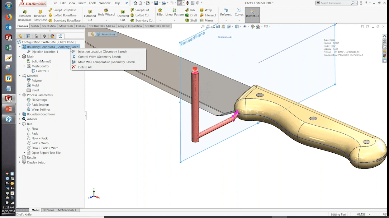
And I’ll go ahead and turn on the SOLIDWORKS Plastics add-in instead. I’m gonna open up this part file that I was working on. This is just a simple kitchen knife, and of course, in this case, it’s got a plastic handle, so I would be molding the plastic handle there around the knife blade itself. It’s kind of an insert over-molding type simulation. And so again, previously if I wanted to do a plastics fill analysis, the first step would always have to be to create the mesh of this part.

Boundary Conditions Geometry-Based Folder

And then after I’ve done the mesh, I can do the rest of the setup. Well, now you’ll see that when you go to create a new plastics project up at the top here, you’re gonna have this new folder called boundary conditions geometry-based. And if I right click on that, you’ll see that I can create a few different things like for example, the injection location, right on the model itself. And that way, it will never have to be redefined just because I wanna change a dimension or change the material or copy the study or things like that.

I can, for example, click this face right there or any other area on the model. And the way I’ve done it in this example over here is I’ve made another configuration where I’ve modeled in the actual runner and gate system. And so now, you can see at the top, I’m able to put in this injection location feature just by clicking on the face. So no more selecting nodes or elements in the mesh. It’s simply linked to that face. And even if I made the screw larger with a bigger diameter, I wouldn’t have to go change this injection location.

The same thing with the mesh controls here. Just like in SOLIDWORKS simulation, if you were doing a stress analysis and you wanna refine the mesh on a particular face, like for example, the gate down here, all I gotta do is click the face, type in the mesh size, and that will stay even if I want to go back and redo the mesh later. I won’t have to refine this again or change with the sizing edge just because I regenerate the mesh.

Geometry-Based Conditions

So, we’ve only got that for a few of the set of conditions right now. And of course, we’ll see in the future how that gets expanded but the other important thing to is that any of these geometry-based conditions are also saved in the SOLIDWORKS part file just like the other simulation tools. So again, if you send this part to somebody else, and you want to make sure that they are using the same gate location, the same mesh controls or low temperatures, those will already be in the part, you won’t have to go and redefine them. What that means is, it’s going to be faster for you to do design comparisons.

Like in this case, I’ve got my gate to sort of in the initial location here, where I’ve got some results I can look at. But if I wanted to find out what the effect would be of moving that gate, again previously, I would have had to go in, change the geometry and then basically re-mesh the whole model and start from scratch.

Duplicate Study

Now, in 2019, I can simply click this button to duplicate the study. I could call this, for example, maybe Gate C, and when I do that, I’m going to get a new study underneath a new configuration here. All the setup is preserved including these set of conditions on the model, which means, even if I go change the geometry, like for example, if I want to move the gate gear down to the end, let’s go ahead and make this larger dimensions evidence towards the other end of the handle.

Now you can see, I moved the entire runner system but my injection location is still where it was, my mesh control is still where it was, and all I need to do is just go in, like this edit solid mesh button, which will regenerate the mesh with all the same mesh settings that I already had before. Then it’s just simply a matter of hitting run.

With that, I’m going to pass it over to Silvio, and he’s going to wrap up with showing the enhancements in SOLIDWORKS Simulation 2019, particularly focused around the topology study, which we introduced last year. Silvio, you should be the presenter now.

SOLIDWORKS Simulation

Thanks, Damon, let me share my screen here. All right, well, you guys should be seeing my SOLIDWORKS Simulation 2019 slide. I’m going to wrap up this presentation here talking about our structural tool, which is SOLIDWORKS simulation and the enhancements that are available to that product.

Nonlinear Analysis

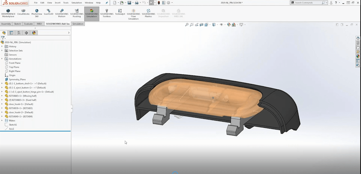
You see that we have a variety of different enhancements here, and this first one that I’m going to discuss, relates to the SOLIDWORKS simulation premium users who do a nonlinear analysis. I’ll be discussing what is available within that product type here. What we’re looking at is a cover assembly. And before I get into actually showing you what the enhancement is, if I refer to the static analysis, if we go back to 2018, SOLIDWORKS gave us this functionality where you see that this cover assembly, if I were to turn off this transparency and show you how this is connected. In real life, there’s an actual pin running through this actual assembly here. And you see that the pin would be running through multiple faces.

Previous Enhancements

So, the enhancement that SOLIDWORKS gave us in 2018, specifically for linear static frequency buckling, or even linear dynamic study types. It gave us the functionality to get into the connection and define a pin connector and being able to define a multi-faced pit. Where prior to that enhancement, the limitation that we had before was, you only really have the option to select two cylindrical faces from two different bodies. So, you are limited based on the number of faces that you’re able to select and the number of bodies that you are actually connecting these pins with.

The enhancement that they gave us last year was being able to not have to create multiple pin connectors or potentially create a split line feature to separate certain faces into two unique faces to be able to get away with defining a pin through multiple faces like what we see here. So in 2018, they gave us that functionality.

In 2019,  the enhancement is that they gave us that functionality for a nonlinear analysis. So you see that I created this study as a linear static analysis, we can take advantage of the copy study functionality of being able to transfer in are no penetration contacts that include our pin connectors as well, and transfer it to a nonlinear analysis. And when we do that, if I refer to my completed study here, you see that we’re now looking at a nonlinear analysis and our setup is essentially the same where it transferred over our contacts in our pin connector. And you see now that for our pin connector here, again, we’re able to select up to 10 faces to specify that a pin is going through this multi-body assembly. Right? And the real benefit comes from when you actually run the analysis. So, this just makes your life a little bit easier in terms of setup of again, not having to define multiple pin connectors or being able to specify split faces, it allows it to do it in one single shot. And when we actually take a look at the results and load up our connector forces here, you’ll see that we’re able to see the shear forces, the axial forces, the bending moment, the torque. These are the traditional outputs of what you would be able to get from a pin connector or bolt connector. In this case, with the pin connector, since we are defining a multi-faced type of input, you see that these are separated into different sections now, essentially into different joints. And now, since we’re selecting a pain is going through more than one face or more than two faces for more than two components, it’s allowing us to see again, the sheer force, axial force, bending moment and the torque at those individual joints.

So you see that I can just simply click on those joints and it snaps to the neighboring face. We got this new enhancement for 2018 and now it’s available to us for a nonlinear analysis, right? So being able to really view the different outputs at those different faces when we define pin connectors. So, very subtle enhancement there but yet very beneficial if you’re running now a nonlinear analysis. The other enhancement here comes with if you utilize a lot of remote loads.

Remote Loads

Before we get into the actual enhancement, what a remote load is doing is if you take a look at the image here is being able to define a load in a remote location but still have it be linked to the actual model that you run in the analysis on. So let’s say, for instance, that model had some sort of handle or some sort of component that’s imposing a load on the actual geometry that you care about what you want to see stress results and display some results on but you don’t necessarily want to include that model into the analysis.

You can get rid of that model and say that there is this remote location. That we’re applying some sort of loads, some sort of force or a moment that is going to be tied through these rigid bars here onto the actual face. So it’s a nice way for you to simplify the analysis without having to include any components that you don’t necessarily care about. So that is, again, a reminder of what we can do with this remote load mass.

Remote Location

In 2018 and prior to that, this is how the interface looked like where you have to specify if you’re going to do a low direct transfer, or a load or displacement rigid connection. You’re really saying that the loads and the forces and moments that you’re defining at that remote location are being able to transfer uniformly to the actually selected faces. So essentially, you’re transferring those forces and moment onto the faces in which is attached to in order for the model that you’re interested in seeing, being able for it to deform and be able to produce some results. Then the other option that you had there was being able to define a rigid connection, which pretty much means that it’s going to define and specify that these coupling faces or the connected faces are going to be treated as or deform as a rigid body.

There were some assumptions linked to that. Again, like if you were doing a low direct transfer, really, what that’s assuming is that the omitted components are more flexible than the included components that you’re running the analysis on. Because we’re now able to transfer again the forces in moments onto that model, and for it to form in some shape. So really in 2018 and prior to that, what we’re assuming is that those forces and loads are distributed onto the attached face here in a uniform fashion.

Distributed Coupling

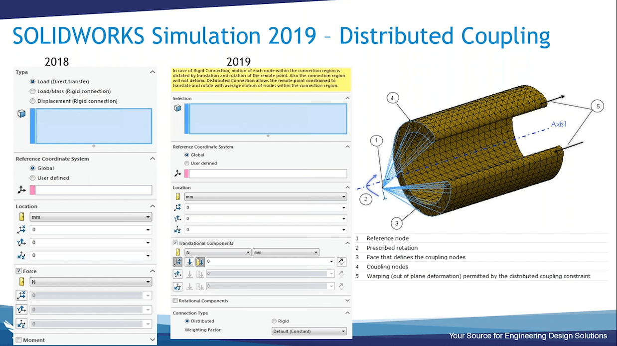
In 2019, you’ll see that the interface, the property manager for remote mass has been slightly updated to accommodate this new functionality of distributed coupling. You see here that on the bottom, we have these connection types, which include these weight factors.

What the enhancement or what distributed coupling is actually doing, is allowing you to select different polynomials or different formulations such as a linear weight factor or a quadratic formulation to be able to define different weight factors that are being distributed on to the actual face.

If we were to specify, let’s say, like a linear or quadratic formulation as far as this weight factor, that weight factor is being applied on that reference point, and then being transferred to the actual coupling space, which is this number four, and it’s now distributing the weight in a different type of formulation versus uniformly, which is what the default option was prior to 2019. And really what the benefit is there with doing that and having that functionality is that we’re now getting a more accurate result in how these forces and moments are being transferred to the actual model.

It’s just a slight enhancement in how those loads are being directly transferred to the actual geometry is the main enhancement there. Of course, if we were to do the rigid connection, which is now located here in this connection type, it’s really just assuming again that the included components are almost stiffer than the omitted ones, and essentially, the entire model is going to deform as a rigid body. So we still have the current functionality of remote mass, but now we have this-this distributed coupling that is able to specify these weight factors,  slightly different from what we could do before.

Topology Study

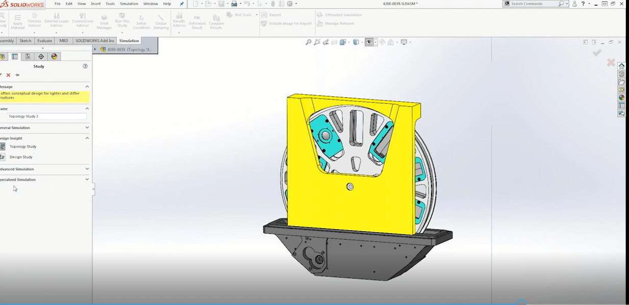
The major change that we have available to us is some enhancements within a topology study. Just to remind you, guys, what is a topology optimization study? Well, for one thing, it was included in 2018 last year, and it was included for Simulation Professional and Simulation Premium seat. And it utilized this SIMULIA Abaqus technology, which SIMULIA Abaqus being our higher level analysis tool to be able to run analysis on a more complicated type of scenario.

It’s utilizing that technique for us to have a baseline design like this hinge, and have the software be able to iterate through our constraints and our goals to be able to reduce the amount of mass being applied onto the model, yet still increasing the stiffness of the geometry. This component is gonna be strong enough relative to how much mass we’re eliminating from the model.

It’s a way to find this optimal shape of a component based on these optimization goals and constraints that you’re able to define, and from there, it’s increasing the stiffness while reducing maybe some displacement, but ultimately reducing the mass. So, that’s what a topology optimization is allowing us to do. And it’s intended for designers who are trying to modify and optimize a current shape to be able to satisfy these design constraints.

And these design constraints that were included in 2018 are the following. You see that the default option here was the best stiffness to weight ratio, which is, being able to specify, “I wanna reduce the amount of weight by 50%” or whatever percentage or try to meet a certain goal, yet still keeping a certain stiffness to the actual geometry for it to essentially – your design constraints.

And it also included manufacturing controls like being able to define preserved regions, which was the lighting phases in the area of the model that you didn’t want the analysis to necessarily get rid of the material. Or specify thickness controls where, again, there’s a certain area in the model that you want to retain, a certain thickness of the geometry, and it also could account for how this model was gonna be extracted from the actual mold if this was gonna be cast or something like that.

Define Goal Constraints

We have a variety of different ways to define these goals constraints and account for these manufacturing conditions in order for us to give us this optimized shape. But this was assuming that we’re only really concerned about purely the strength of the geometry, where it wasn’t really accounting for whether the geometry was gonna be in some sort of vibration environment. When you’re running an analysis where you’re thinking about designing a component, you know, one of the environments that it might be in is some sort of shaky environment where it’s vibrating, or essentially, you want to check where it’s not, that the resonant frequencies don’t coincide with what input is that’s what causing this vibration because that may cause some sort of issue.

Frequency Constraints

In 2019, the topology analysis is allowing you to define this frequency constraint. So in addition to the inputs that we have discussed as far as the stiffness to mass ratio all those manufacturing controls, we can also add that we don’t want the first natural frequency to go beyond or you know, maybe they wanted to exceed a certain frequency value. And this will again tie-in that you want to avoid a certain frequency range, a critical range that you don’t want this to resonate in.

One of the things that many students have asked me in regards to this new tool is, can we specifically say, “I wanna optimized to a certain factor or safety or a certain stress,” and now with 2019, we have that capability. So in addition to what we just discussed, we can specifically say, “I want my overall stress to be, you know, some factor of what the yield strength is to ultimately be under what that yield strength is. You know, for it not to go above yield.

Or, we can specifically say, “I want my factor of safety to be, you know, two times or whatever it may be, right?” So now we can define specifically say, “These are my design constraint. This is where I want my stress to be, and it will run this topology optimization to account for these conditions.” So let’s take a look at how that looks. So, right now, if I go into that model which we’re looking at this assembly now.

There are a couple different ways you can approach this. You can go straight to a topology analysis. After you turn on the analysis, you can go to new study, and you can go in straight up run a topology optimization study. You know, my recommendation is for you to run a linear static analysis on the parent model, which is gonna be that yellow piece that’s now isolated into this component here.

There’s a lot of mass happening there. And ultimately, what I want to know is, can I reduce the level of material that’s in that model to be able to satisfy certain design constraints? So in 2018, those design constraint again included manufacturing goals or including that stiffness to mass ratio. And that’s what we define here. So we essentially said that for our constraint, we wanted to reduce the mass by 70%. And now the only condition that we defined in terms of changing the actual mass parameter. And then we also included that this is gonna preserve. We wanna preserve a certain wall thickness in certain areas of the model, and we want to keep it pretty much no more there or no less than 20 millimeters across the entire model.

When we run the analysis there, the output that we get is pretty much a display of the areas of the model there in which you can remove material, and it overlays that with the outline of what the original model looks like. So you see, with the original model here what this plot is actually showing us, are all the areas that we need to keep within the model for it to still kinda create this level of stiffness that we need based on the load conditions that we applied within the model as well.

You still cut up the problem like, what forces this is gonna endure in addition to those constraints. And you see that from there, it’s saying that we can minimize this model to a certain shape like this, and it still will meet our design constraint. So this is what we were able to do with 2018. But with 2019 now adding in the functionality of being able to account for how this is going to vibrate or trying to avoid certain natural frequency, you see that we can still include, how much we want to reduce this by or want to reduce the mass by 70%. But now we can include this functionality where we can specify that the first natural frequency here needs to be greater than 150 Hertz. So, what that’s saying is that we want to avoid any resonant frequency that’s below 150. So as long as it’s above this 150-mark, then our design will be considered okay where that’s going to follow our design constraint where it’s out of that critical resonant frequency range.

In a combination of that, we can run that and also again and account for that condition, and you see that the result here is gonna be very similar, but you see that it slightly changes where now we can maybe reduce a little bit more, uh, more material in these areas here. We get a slightly different shape. So, now that it’s accounting for this extra condition, you can be a little bit more confident that not only is it going to survive your stress conditions, but it’s also going to survive your vibration conditions that you may have within the model itself, okay?

And then as a reminder of what you can do with this result here is being able to export this into some sort of a condition where, uh, you can either get a graphical representation or export this as a solid or surface geometry to get something similar to this here where if I activate a configuration that included, uh, my model here, uh, bear with me, let’s see if I have one here. So you see that the output that we get from this is this mesh condition where really what– how you use this geometry is we overlay it, we use it as a trace configuration where we can now design a new part that references the areas of the model that we can eliminate.

So I would throw this into or use this model as a kind of a trace to kinda get an idea of how I can reduce that original plate to this now optimized shape, and then I would rerun the analysis to make sure that it’s actually following our stress constraint that we’ve defined originally. Right? But at the end of the day, this is a design tool to help guide you to figure out this optimized shape based on these different strength conditions.

In conclusion, there are some very exciting enhancements for 2019 specifically for the topology optimization there but hopefully, you guys enjoyed the enhancements for all products that involved the analysis tools SOLIDWORKS flow simulation, plastic and the structural tool here. If you would like more information on these enhancements or products, CONTACT US Today! We’ll put you in touch with one of our engineering experts in your area.