As any engineer or analyst working in the field of process piping would know,
it’s necessary to ensure your design meets the local code requirements. Doing
so may prove to be tedious or time-consuming when you aren’t using the right
tools. Of course, SOLIDWORKS has a variety of integrated stress analysis
capabilities that help any designer predict failures such as yielding,
fatigue, or even cracking- from the first concept to final candidate.
 |
But oftentimes, deciding on assumptions for such an analysis can be the
hardest part of the setup. Are the pressures uniform on the inside of the
pipe? Will it be hot enough to worry about thermal expansion? Luckily, we can
simulate the flow of water, natural gas, or other fluids directly using
SOLIDWORKS Flow Simulation- the built-in Computational Fluid Dynamics tool for
SOLIDWORKS- with the added benefit of directly sending these results to your
stress analyses to speed setup time and improve realism.
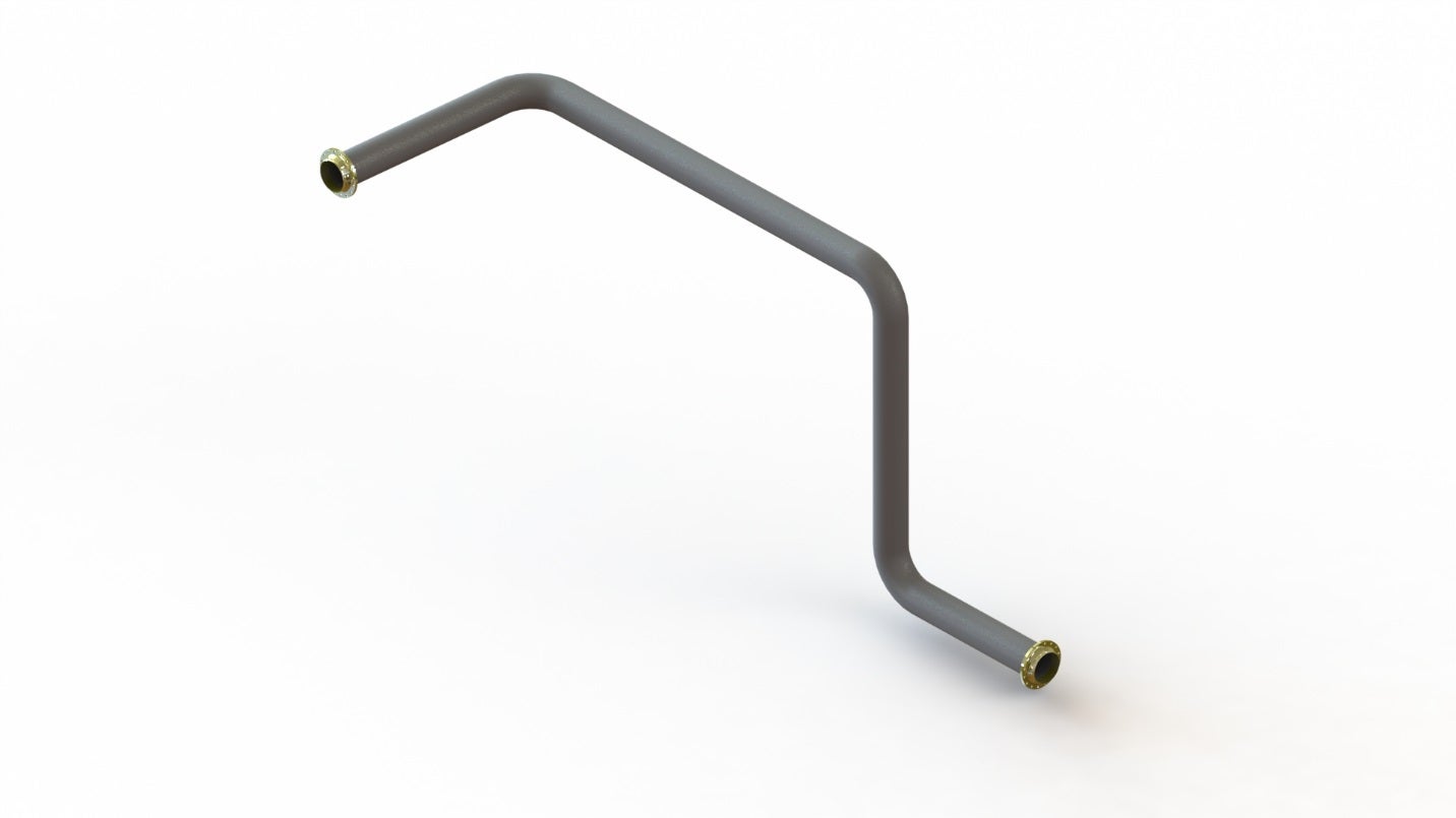
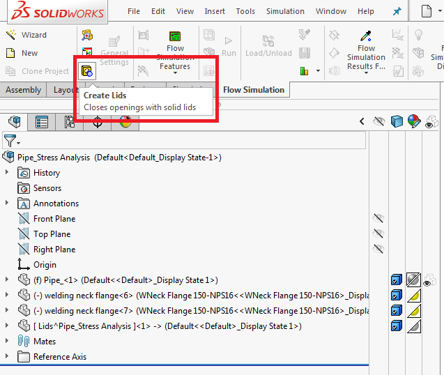
Analyzing a design with SOLIDWORKS Flow Simulation requires very little
preparation- the only requirement for an internal analysis (such as a pipe or
tank) is to close off any openings in the model. This is can be done by
creating parts, or automatically with the built-in Create
Lids tool:
 |
 |
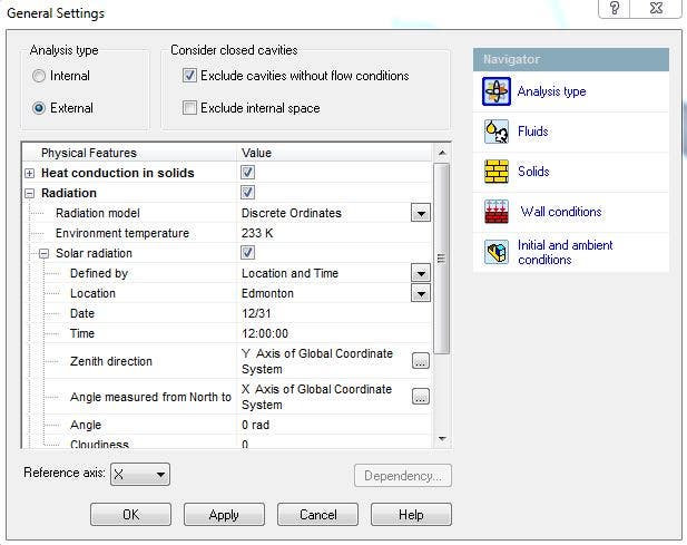
Even though we will be defining the internal flow conditions of the slurry
within the pipe, the study type will be External so that we can also simulate
the heated air coming off of the pipe, which will further improve the realism
of the pipe temperatures- that makes activating
Heat conduction in solids is a must. Radiation may also play a role
so, just to be safe, we can activate solar radiation and simply
select our location, date, and time from the database to give the simulation
the accurate intensity and vector of sunlight.
 |
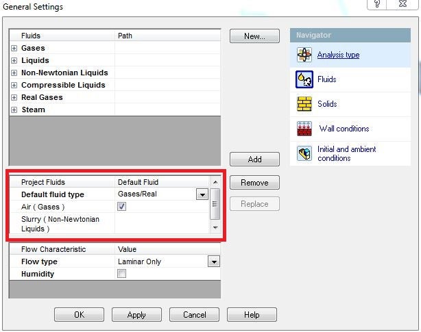
Next, we define our working fluids. Setting Air as the default will
automatically set it as the ambient (external) fluid. Meanwhile, the pipe will
be carrying a mixture of oil & mud, which we can accurately simulate as a
non-Newtonian fluid in Flow Simulation with the built-in item named “Slurry.”
These fluids change viscosity depending on their shear rate, and can’t be
represented properly with a regular liquid model (compressible or otherwise).
 |
To ensure accurate temperatures, we’ll need to define both the pipe material
and the emissivity of the outer surfaces (for radiative properties), in this
case with one of the Steel definitions from the engineering database.
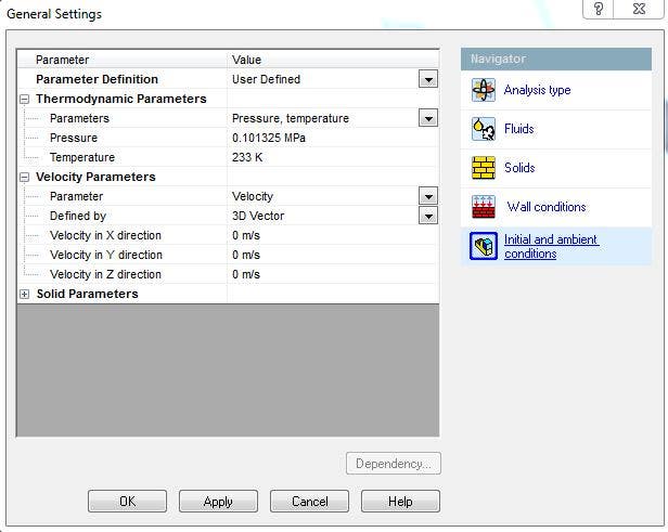
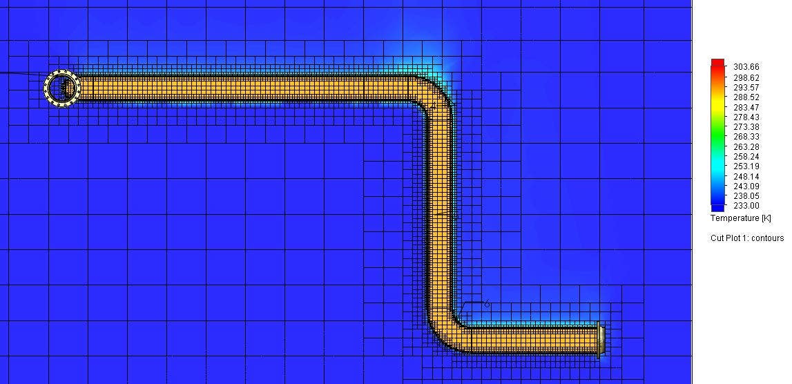
Finally, our ambient conditions will be default except for the temperature,
which will be set at 233 K (-40 F) to mimic a frigid Edmonton afternoon.
 |
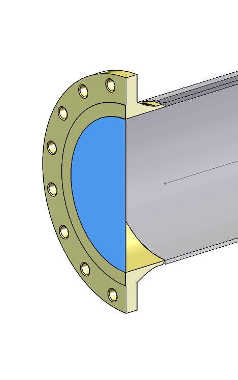
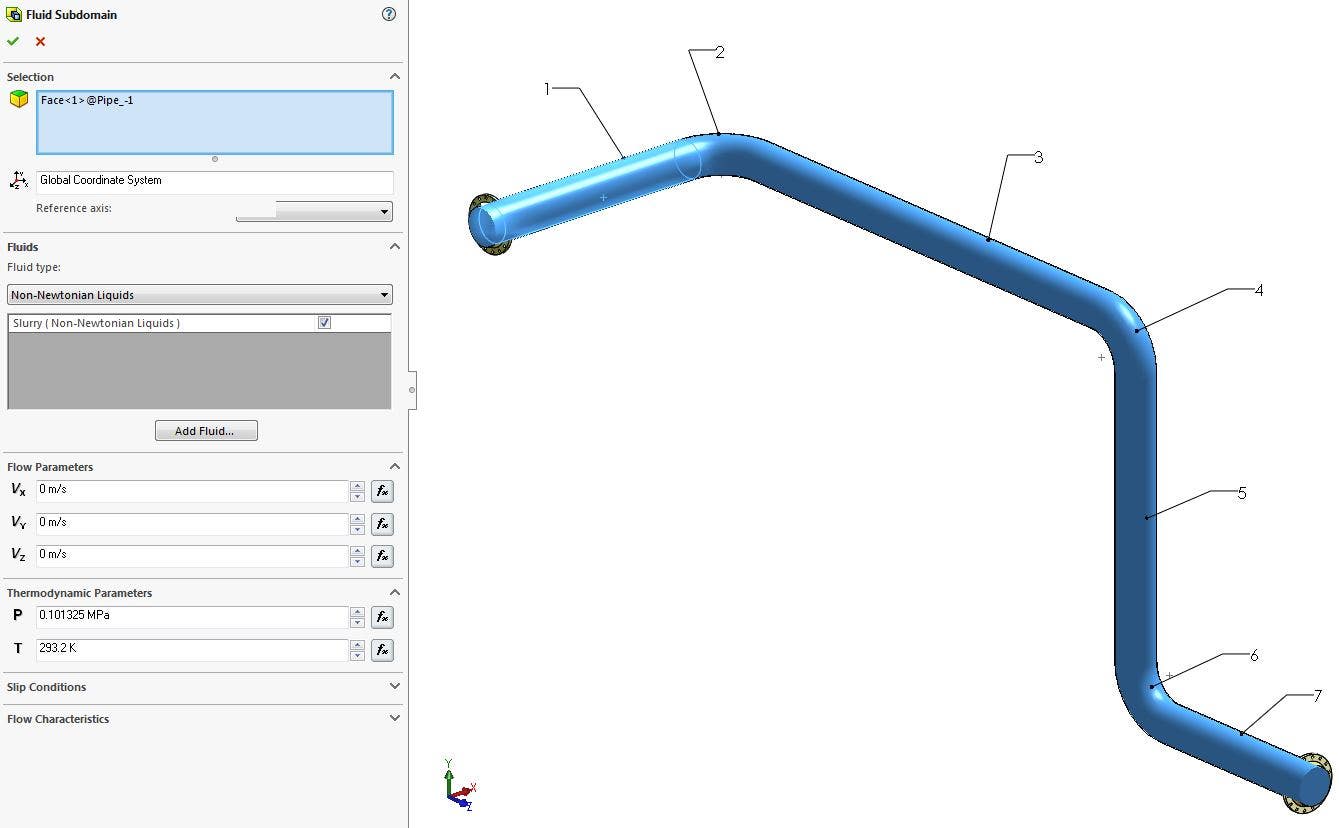
Once the Wizard is complete, we can proceed with the detailed setup. We need
to define a Fluid Subdomain to represent the insides of the pipe
where we have the slurry flowing as opposed to air. We simply need to select
the inner surface of the pipe, and SOLIDWORKS will solve for the fluid region
based on the enclosed volume. The only thing left is to input the
thermodynamic parameters, the assumption here being that the slurry is
extracted from a warmer location.
 |
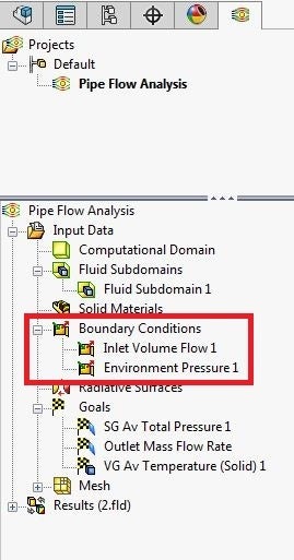
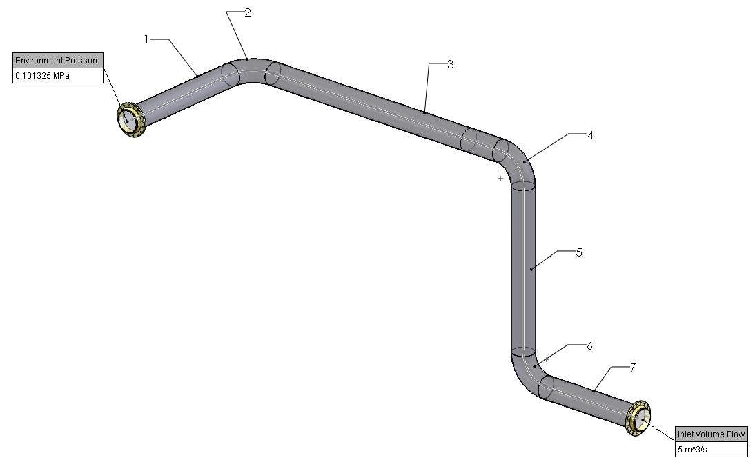
Now, the inlet and outlet conditions can be defined by selecting the inner
faces of the lids: an exaggerated Volume Flow Rate of 5 m^3/s at the inlet,
and Environmental Pressure at the outlet which would represent no further back
pressure in the pipe.
At this point, all physical conditions have been defined. However, we can also
input some items called Goals, which are sensors for the key results we’re
most interested in from the simulation. This makes it quick to check that all
our requirements are being met, even before the simulation is complete and
also helps ensure that we’ve found convergence, or the true steady-state
results, which has traditionally been a challenge with CFD tools. Here, we’ve
defined goals for the mass flow rate, inlet pressure, and temperature.
 |
 |
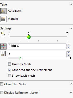
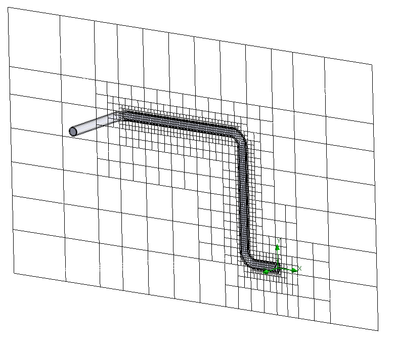
The biggest time saver with SOLIDWORKS Flow Simulation is the automated
Cartesian mesh technology, which quickly generates the mesh for almost any
input geometry with even the default settings. While there are many options
available for manual mesh refinement, in this case, we can get acceptable
accuracy by simply entering in the size of the channel that needs to be
captured (the ID of the pipe), and check the “Advanced channel refinement”
option:
 |
 |
At this point, we can run our analysis either on the local machine or a
networked computer. When complete, we get our key results right away from the
Engineering Goals table.
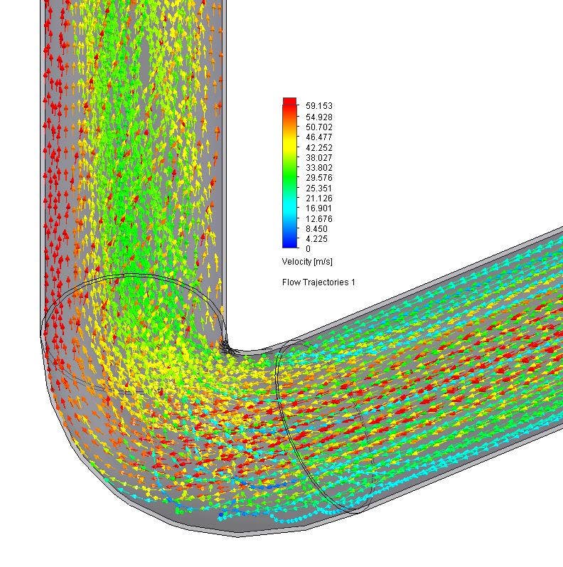 |
Finally, Flow Simulation’s array of visual results like Flow Trajectories and
Cut plots can help determine qualitatively why a design is behaving the way it
is, and how it might be improved.
 |
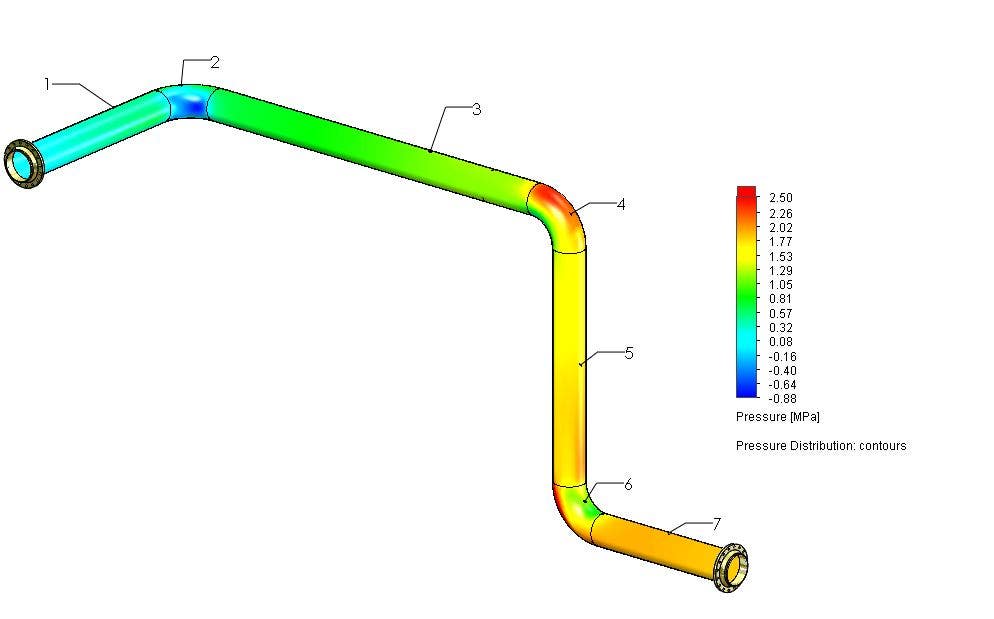 |
If we’re satisfied with the performance of this pipe from a flow perspective,
we can proceed to look at a plot of pressure on the inner walls of the pipe,
and export those directly to SOLIDWORKS Simulation for stress analysis.
|
|
With the Simulation add-in enabled, we can create a Static analysis, and
automatically import these pressures and temperatures to the study in order to
find the stress and deformation of the pipe:
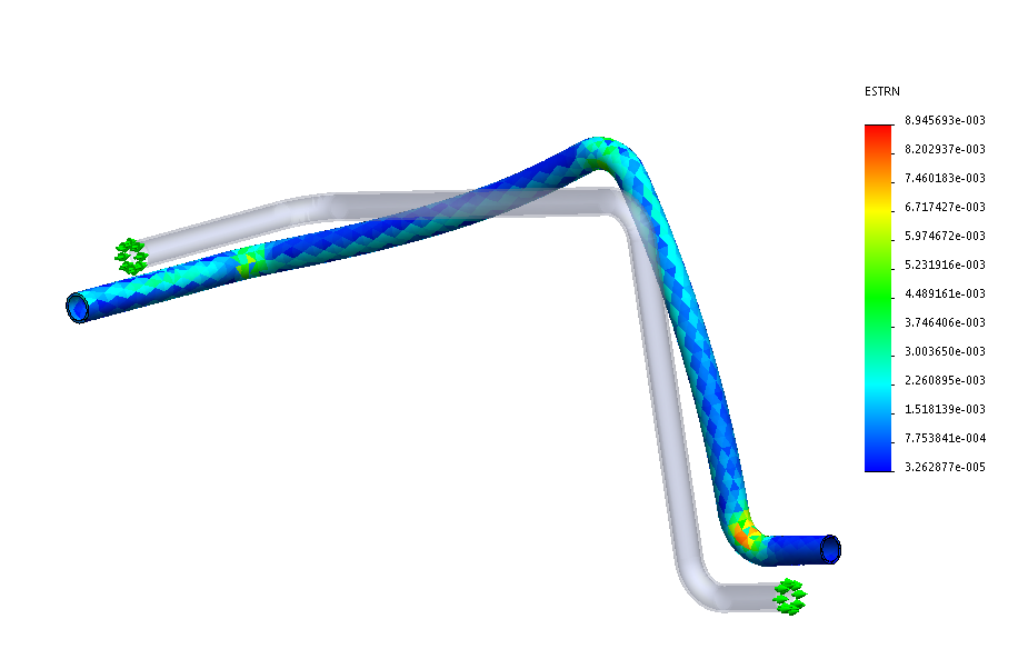 |
We can see some significant strain and deformation in this pipe, so at this
point, it may be wise to use a heavier gauge or stronger steel. Luckily, the
process is a simple as changing the dimension(s) in SOLIDWORKS and re-running
the analyses. With an integrated process like this (with optional data
management solutions like PDM Professional), the jobs of pipe designer, fluids
expert, and stress analyst can be done at once, with rapid iterations, leading
to a much more robust and optimized design before a prototype is ever built.
Keep following the Hawk Ridge Systems blocks for more examples of how the
tools and services we offer can have a similar effect on your design process.
For more information, check out our
YouTube channel
or contact us at
Hawk Ridge Systems
today. Thanks for reading!