Whether you are designing electric motors or high-voltage equipment, low-frequency electromagnetic simulation can help improve designs and even find problems before they occur in the field.
The range of applications for electromagnetic simulation is practically unlimited, but in general, we can break down this type of analysis into two main groups: low and high frequencies.
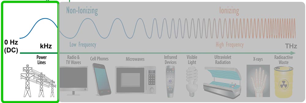
In this blog, we’ll focus on the 0 Hz to 1 kHz range on the electromagnetic spectrum, exploring a brief overview of the power that SIMULIA CST Studio Suite offers for devices operating in the lower range of the spectrum. SIMULIA CST has solutions to simulate any emag problem, from DC to light, all within a clean user interface.
The Difference Between High- and Low-Frequency Simulation
High-frequency simulation tends to focus on signal integrity, such as S-parameters or field patterns of an antenna array broadcasting in the GHz range.
Examples of high-frequency simulation are antennas, radars and high-speed digital and high-performance communication components, which are where most people consider simulation useful, especially in the ever-changing world of connected devices.
However, the lower frequency range introduces a host of new criteria for validation and improvement, particularly for products that rely on generating magnetic fields for their operation. Low-frequency simulations focus more on results such as field strength, forces and charges that are typically found in electric motors instead of signal integrity.
SIMULIA CST Studio Suite as a Low-Frequency Simulation Tool
SIMULIA CST Studio Suite has a host of solvers that can fit your application. You can use SIMULIA CST’s project template to help you choose the right solver.
Templates can help guide you through the simulation setup based on the product and problem type. The wizard suggests relevant solvers, mesh, monitors and more.
Start with the type of simulation. We’ll use “Statics / Low Frequency” for this blog.
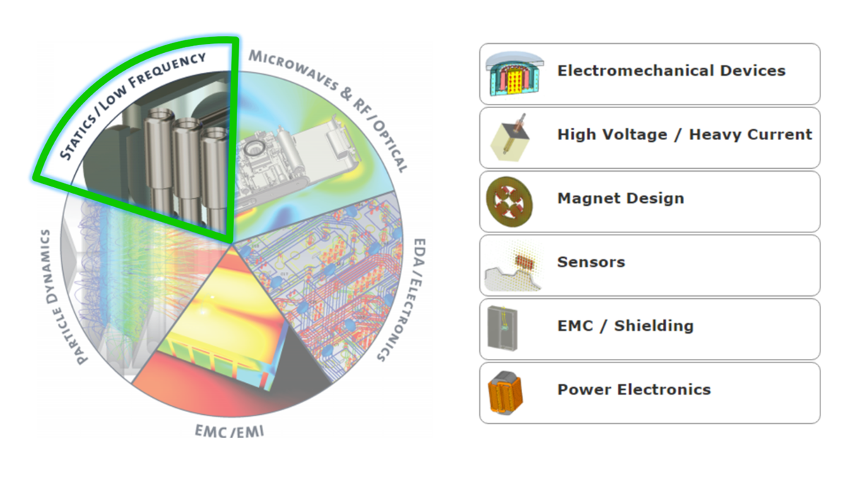
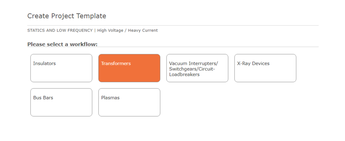
Then on the menu to the right, you’ll choose one of the workflows. For this blog, we’ll choose “High Voltage / Heavy Current.”
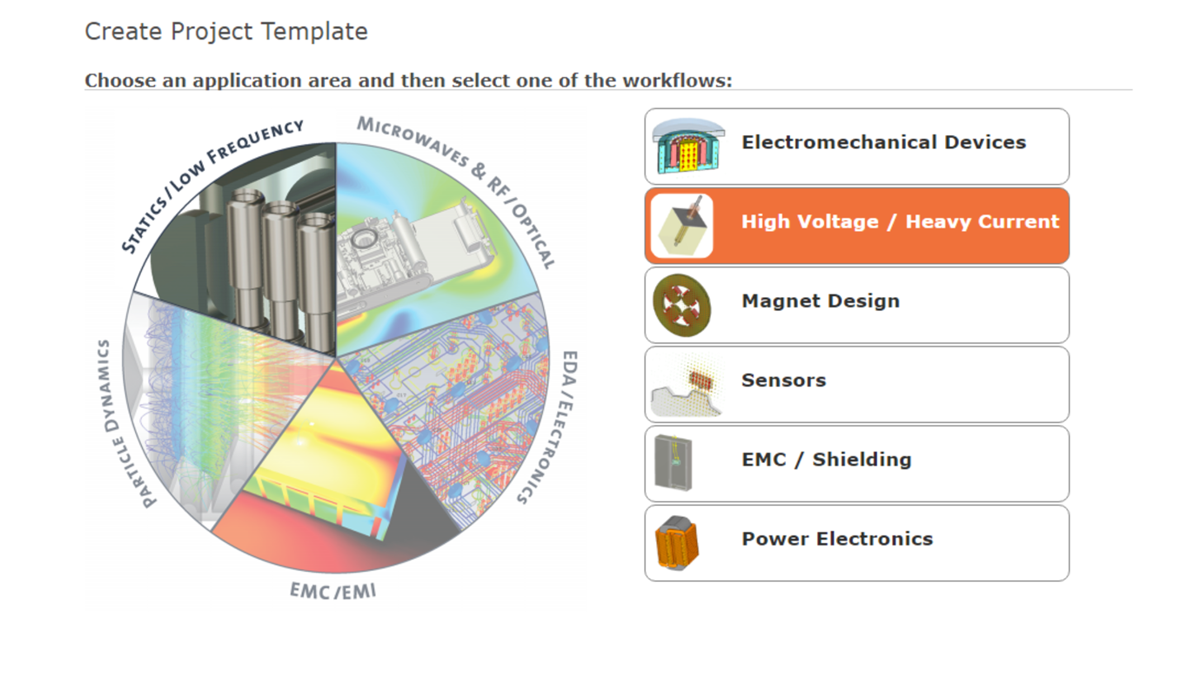
From there, you can choose a more specific workflow. After choosing “Statics and Low Frequency” and “High Voltage / Heavy Current,” we’ll choose “Transformers” for our workflow.
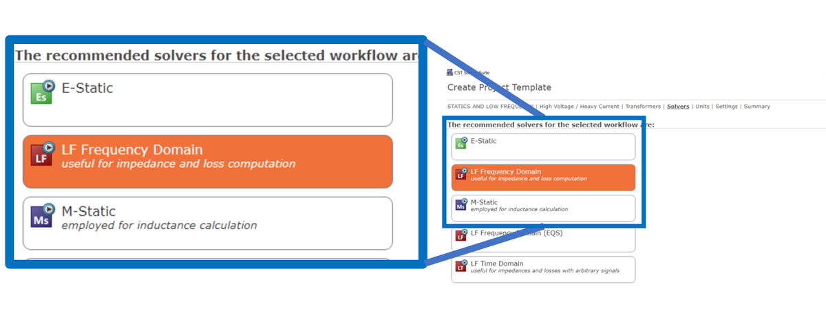
After choosing your specific workflow, the template will recommend a solver for your simulation. The template recommends a dynamic solver, LF Frequency Domain.
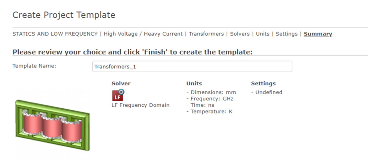
The last menu will give you a summary of your choices to review and finalize the template. Our selection summary shows “Statics and Low Frequency” and “High Voltage / Heavy Current” with units in mm, frequency in GHz, time in ns and temperature in Kelvin (K).
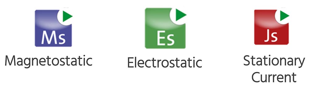
3 Types of Static Solvers
Starting with statics in SIMULIA CST — that is, products that operate mainly on DC current, they don’t take time-dependent aspects into account and assume a steady state.
Applications that can benefit from this type of analysis include:
- Magnetic sensors (Magnetostatic solver)
- High voltage terminals (Electrostatic solver)
- Circuit breakers (Stationary current solver)
In each of these analyses, you can define the source, boundary conditions and other workflows in SIMULIA CST’s complete user environment, which integrates meshing, solving and reviewing results.
Below is an example of a magnetic Hall sensor where we review the steps to define permanent magnets, perform parameter sweeps, review force measurements and show 2D/3D results of the magnetic forces.
2 Types of Dynamic Solvers
We can also look at some dynamic systems using those building blocks, such as defining magnets and coils as sources.
In SIMULIA CST, dynamic solvers take time-dependent aspects into account, unlike static solvers. They include:
- LF Frequency Domain (Magnetoquasistatic, electroquasistatic or full wave)
- LF Time Domain (Magnetoquasistatic or electroquasistatic)

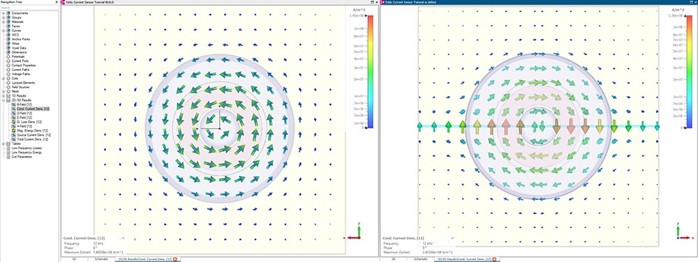
Simulating non-destructive testing (NDT) using an eddy current sensor shows how a current-driven coil can detect a defect in a metal slab. The sensor works by inducing an electromagnetic field very close to the surface of a metallic object.
Any variations, such as gaps or cracks, in the structure will create variations in the current fields, which can be analyzed to determine the location and size of the feature.
Below is a screenshot showing the top view of a coil sensor structure and a metallic plate using the magnetoquasistatic option of the LF Frequency domain solver.
You can see the conduction current density arrow pod and coil voltage frequency. On the left, there is no defect, and on the right, there is a defect, which is shown by the variation in the current density and direction.
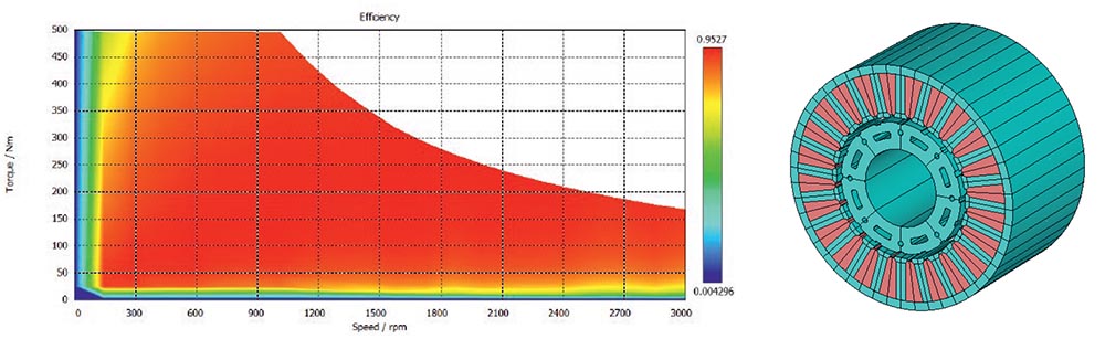
Combining permanent magnets, coils and motion, we can simulate and optimize electrical machines, like a motor. The ability to simulate complex tasks within SIMULIA CST, such as machine tasks and co-simulations with different solvers, allows you to analyze a wide range of results — all within a simple interface.
Below, we simulate an electrical machine using the LF Time Domain solver. We can review important results for motor design like efficiency plots, forces, torque and more.
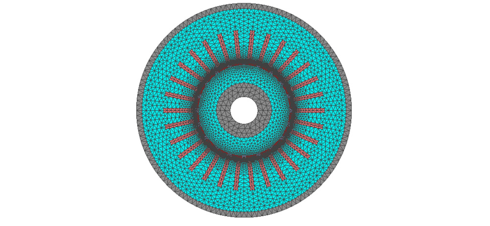
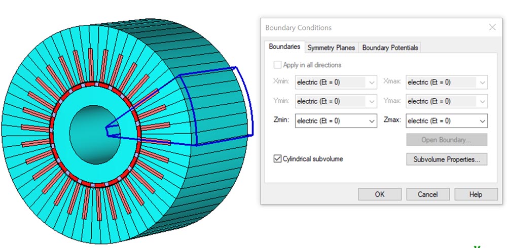
SIMULIA CST has various tools to help reduce the complexity of simulations like this motor using planar mesh and sectional boundaries. Both techniques create a simplified structure to reduce the computational load for simulation while still giving the same results.
Below, you can see we used the planar mesh in the first image, and in the second image, we used the sectional boundaries.
The Final Note
SIMULIA CST is a powerful solution for low-frequency simulations and other emag challenges and applications.
For more info, check out our webinar on lesser-known low-frequency capabilities in SIMULIA CST, where we dive deeper into these low-frequency applications and the rest of the SIMULIA CST capabilities. Thanks for reading!
If you have any questions about SIMULIA CST Studio Suite and low-frequency simulations, contact us at Hawk Ridge Systems.