SOLIDWORKS Simulation: Finding Accurate Stress Results with Singularities Part 1

Introduction

Stress singularities are an unavoidable occurrence in any theory of elasticity regardless if the calculations are done by hand or simulated using software. An artificial stress concentration occurs in areas where a sharp corner is created and is sometimes unavoidable no matter what simplifications you do to the geometry.  In this blog I am going to show you a method to determine the reach of the stress singularity and a safe distance when you can begin to trust your results.

(click here for more information about stress singularities and convergence)

Procedure

In order to determine the validity of the results I am going to do a convergence test on nodes in the area of the stress singularity and see how far the singularity effects. Usually when you refine the mesh the location and assigned number of a node changes so I set up a grid system using split faces and put sensors on the vertices of the grid. This forces a node in the corner of the grid and the sensor ensures that I am getting the stress results at the same location every time regardless of the mesh density and shape. The split faces in the grid are a double blessing because I can use a mesh control on the grid entities to refine the mesh only in the area I am recording data. Once I have my results from multiple studies with different mesh densities I will compare the stress results from each sensor, look for convergence and determine the validity of the data at that location.

Example 1: Two Parts Contacting

Location of Singularity

For this example I am not going to waste time explaining the boundary conditions and contacts and only focus on the stress concentration itself because I want to have one for this example. As you can see in Figure 1 and Figure 2 a sharp corner is created right where the upper part leaves the bottom part even though the bottom part has a fillet.

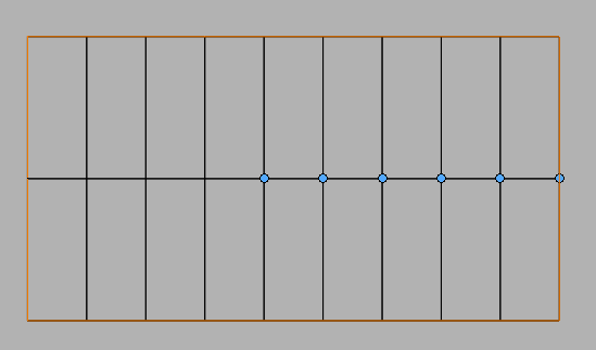
Set up of Grid and Sensors

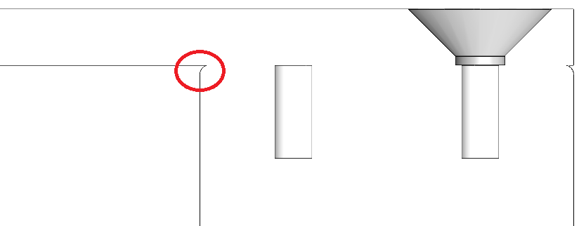
To create the grid I started with a sketch on the face that held the stress concentration. I sketched a rectangle around the stress concentration then used the segment tool to split the lines into equal segments then inserted lines to create the grid. The linear pattern tool could also be used for the same affect. Once I had the sketch I used the split line tool to project the sketch onto the face resulting in multiple faces, lines, and vertices that I am able to select for my sensors and mesh controls.  I placed 6 sensors on inner vertices so I can get consistent readings in those locations. I named each sensor the relative distance they were from the edge of the grid with the names “Outside”, “0.02 in”, “0.04 in” etc.

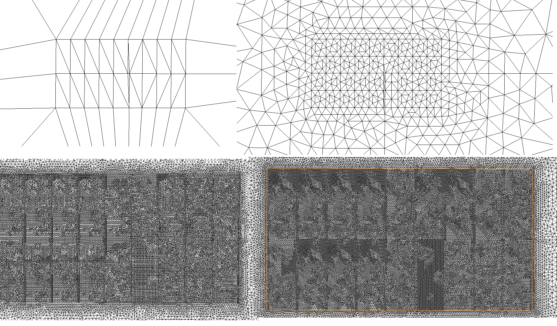
Mesh Refinements

For the convergence test I used 4 different meshes with a varying mesh control applied to the faces on the sensor grid. As the mesh is refined more elements are added to the grid increasing the amount of elements, nodes and the total degrees of freedom in the system. Figure 4 shows graphically the intensity of the mesh in the 4 runs and Table 1 lists the degrees of freedom in each study. The mesh control was increased by an order of magnitude between the final 3 runs (0.1, 0.01, 0.001) in

Table 1: Degrees of Freedom in the Entire System for Each Mesh Refinement

	Run 1	Run 2	Run 3	Run 4
DOF	277062	399885	1483434	1628157

Results

First Run

The first mesh was rather coarse in regards to the sensor grid with only 2 elements per grid square. The stress values at the sensor locations are shown in Table 2. This is a big discrepancy in such a small area so some mesh refinement was definitely needed.

Sensor	Von Mises Stress (MPa)
Outside	6.66929
0.02 in	7.30394
0.04 in	7.34552
0.06 in	11.0647
0.08 in	17.3569
0.1 in	65.4597
Max	116.959

Table 2: Von Mises Stress at Sensor Location for the First Run

 

Second Run

The second mesh has 14 elements per grid square and tells a different story. All of the stress values are higher as shown in Table 3.

Sensor	Von Mises Stress (MPa)
Outside	15.0691
0.02 in	15.9168
0.04 in	17.2586
0.06 in	19.6129
0.08 in	23.6242
0.1 in	111.182
Max	233.795

Table 3: Von Mises Stress at Sensor Location for the Second Run

 

Third Run

The third mesh has a significant refinement and I don’t even want to try and count the number of elements in each grid. The degrees of freedom increased by 270 percent but most of the stresses only increased by under 10 percent. This is a sign that the values are converging. The recorded values at each sensor location for the third run are shown in Table 4.

Sensor	Von Mises Stress (MPa)
Outside	15.0539
0.02 in	15.738
0.04 in	16.7172
0.06 in	18.4528
0.08 in	22.5707
0.1 in	80.1137
Max	622.995

Table 4: Von Mises Stress at Sensor Location for the Third Run

 

Fourth Run

The fourth and final run only saw an increase in the degrees of freedom by 10 percent but the stress at the singularity location changed by more than that. Most of the sensors on the other hand changed by less than 1 percent and taking into consideration the significant digits of the input load there was no change at all.

Sensor	Von Mises Stress (MPa)
Outside	15.0219
0.02 in	15.7525
0.04 in	16.8399
0.06 in	18.6981
0.08 in	23.0476
0.1 in	75.7974
Max	532.041

Table 5: Von Mises Stress at Sensor Location for the Fourth Run

Graphical Results

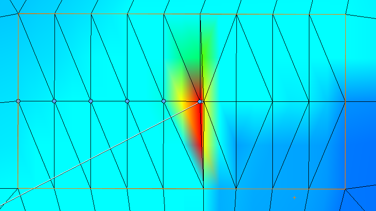
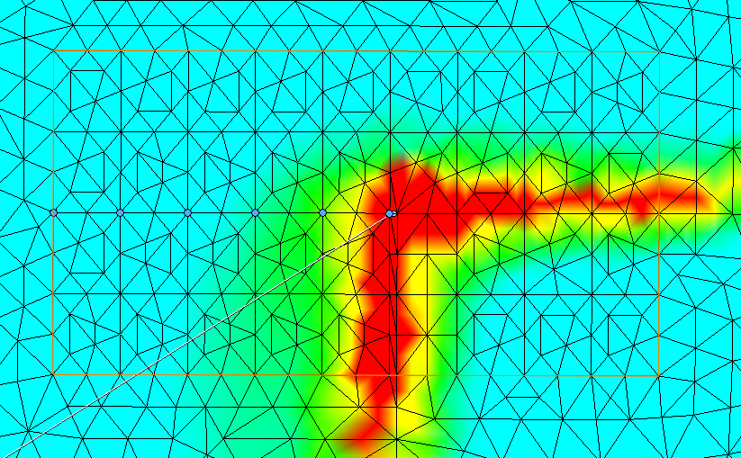
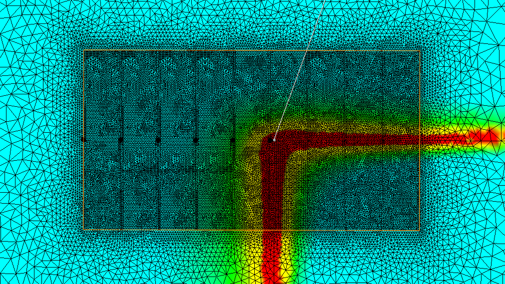
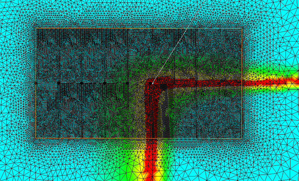
Figure 5 through Figure 8 is a graphical representation of the Von Mises stress in the grid. The Grid is outlined in orange and the sensors are emphasized by a blue or black dot. The red colour of the plot has been set to the material yield strength. As the mesh is refined we can see the stress push outward and then become more defined and have discrete boundaries. We can also see that most of our sensors are below yield so the values are within the assumptions of a static study.

Convergence Plots

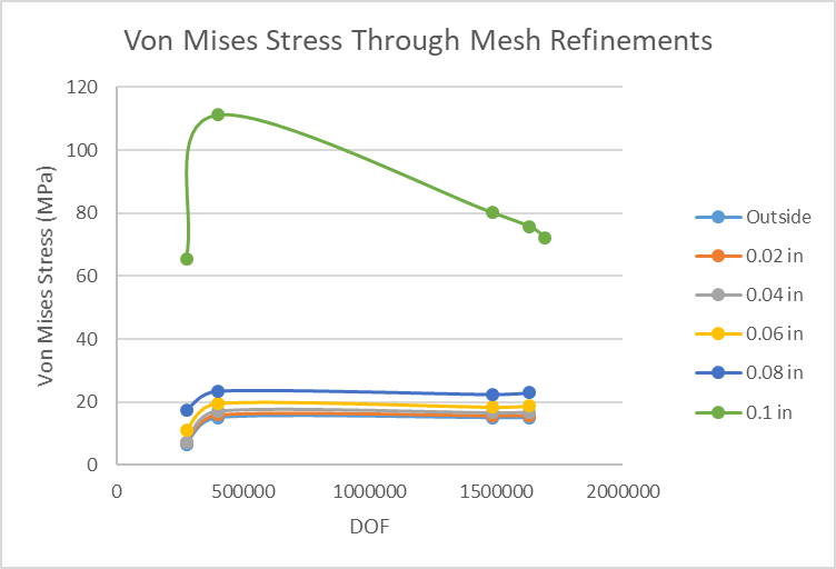
As we can see in in Figure 9 all the stresses increased after the first refinement and the majority of them converged after continued mesh refinement. The sensor located 0.1 in from the outside tells a different story. The value tends to have a rather linear decrease with each mesh refinement and adding another data point to that is further evidence that the sensor is not converging. With more mesh refinement we might be able to get the value to converge but I am very close to maxing out my hardware while creating my mesh.

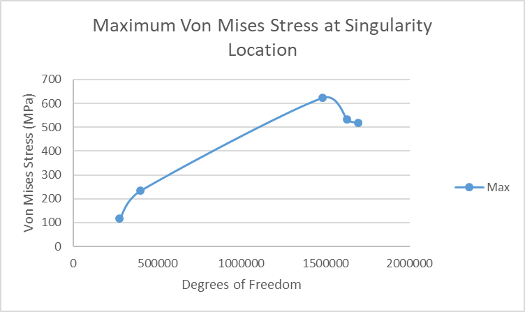
I left the singularity in its own plot because the high stress values would have distorted the plot of the other sensors. As we can see in Figure 10 we get a very large increase in stress with the increase in the degrees of freedom and reduction of element size. This points towards a mathematical singularity.

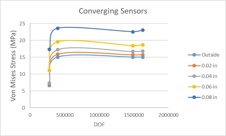
Figure 11 is a plot with a better resolution for the sensors that experience convergence. With this plot we can also see the trend of how the stress decreases as it moves away from the singularity. Again remember that I named my sensors by their distance from the outside of the grid, meaning the bigger the number the closer to the singularity they are.

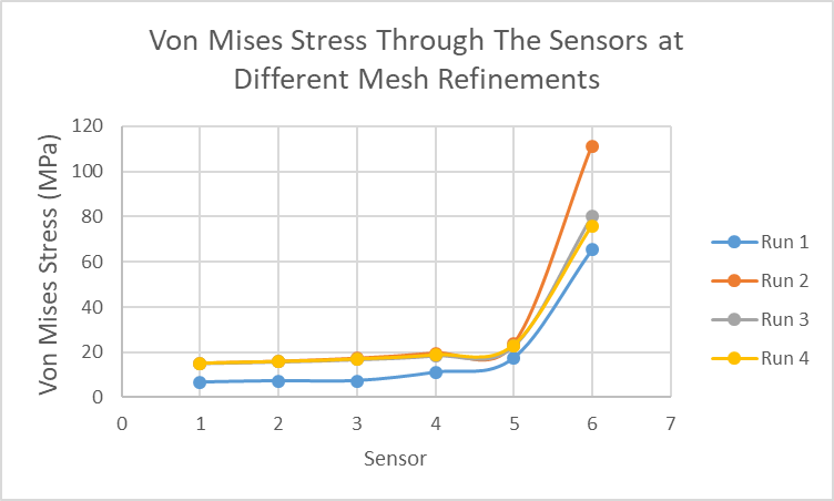
Figure 12 is another way of visualizing convergence. The x axis represents the sensors and the y axis is the stress experienced for each run. We can see that the stresses for runs 2, 3, and 4 are almost identical for the first 5 sensors which converge but split apart at the sixth sensor. The sixth sensor or sensor 0.1 in seems like it is converging around the 80 MPa mark but further data would be needed to confirm that.

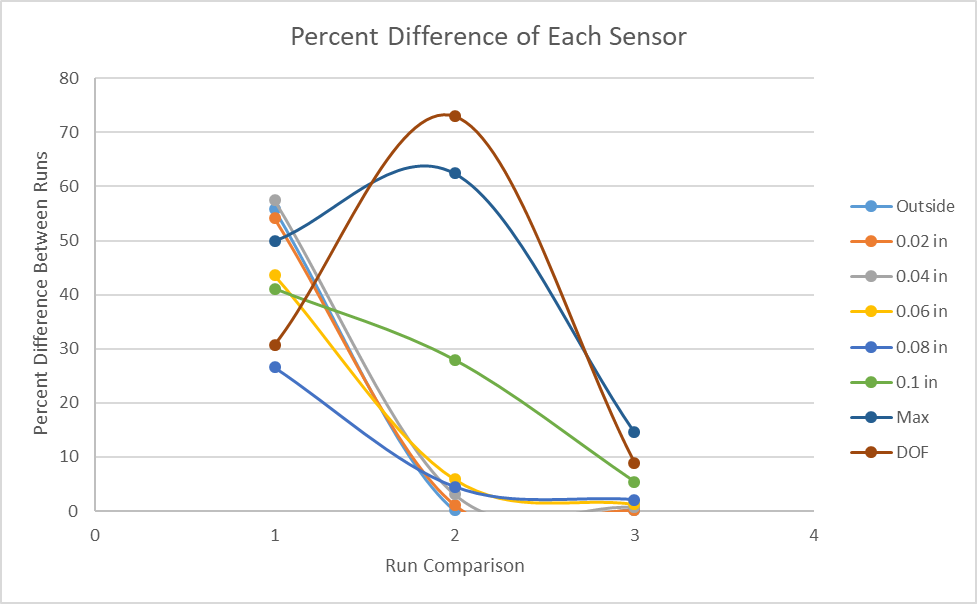
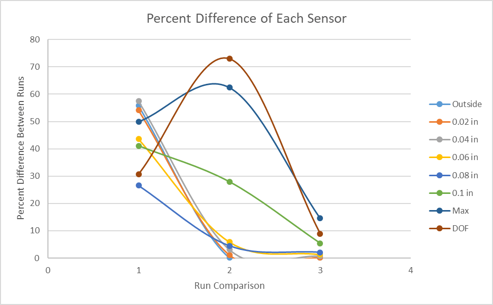
Figure 13 is the percent difference calculated between each run for the sensors and degrees of freedom. Point 1 on the x axis is the difference between runs 1 and 2, point 2 is the difference between runs 2 and 3, and point 3 is the difference between runs 3 and 4. At point 2 we can see a massive change in the degrees of freedom but a very small change in the converging sensors. The data used to create the plot is shown in Table 6 to better understand the plot.

Table 6: Percent Difference of Von Mises Stress and Degrees of Freedom for Successive Runs

	Percent Difference
Sensor	Run 1-2	Run 2-3	Run 3-4
Outside	125.95	0.10	0.21
0.02 in	117.92	1.12	0.09
0.04 in	134.95	3.14	0.73
0.06 in	77.26	5.91	1.33
0.08 in	36.11	4.46	2.11
0.1 in	69.85	27.94	5.39
Max	99.89	166.47	14.60
DOF	44.33	270.97	9.76

Conclusion

So I can conclude that the first 5 sensors are converging and the stress results displayed are independent of the mesh. As an aside there is a negligible difference between the nodal and elemental solution in the region of the sensors giving me further confidence in the results. Sensor 0.1 seems to be tending to converge but since it is over the material yield strength the exact value is obsolete as we are in a linear study.

Table 7: Distance Sensor is From Singularity and if Convergence is Reached

Sensor	Distance From Max Stress (in)	Distance From Max Stress (mm)	Converged
0.1	0.0011	0.028	no
0.08	0.0214	0.543	yes
0.06	0.0417	1.059	yes
0.04	0.0620	1.574	yes
0.02	0.0822	2.089	yes
Outside	0.1025	2.604	yes

So as we can see we were getting converged results half a millimeter or two thousandths of an inch from the singularity location.  Now that is really close but I am going to do another test on a different singularity and try to replicate my results. This blog is continued in Part 2.

For more information, check out our YouTube channel, get a SOLIDWORKS Simulation quote or contact us at Hawk Ridge Systems today. Thanks for reading!