In this video and blog, we take a look at a conjugate heat transfer problem
with both convection and conduction using
SOLIDWORKS Flow Simulation.
Here are the steps used to set up the analysis.
Flow Simulation is a computational fluid dynamics (CFD) tool that operates
directly inside of SOLIDWORKS. You’ll need both
SOLIDWORKS and SOLIDWORKS Flow Simulation installed, with the Flow Simulation add-in
enabled, to follow along with this guide.
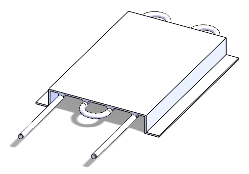
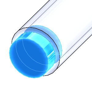
The first step is to get the geometry ready. For this cold plate, lids are
needed at both ends of the cooling tube. This allows the inside of the tube to
be defined as a separate internal fluid volume.
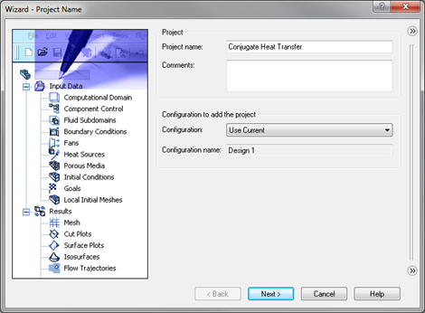
Next, I’ll create the Flow Simulation project using the Wizard. From the
Flow Simulation menu, I’ll select Project, Wizard. I’ll name the
project “Conjugate Heat Transfer” and choose to use the current configuration.
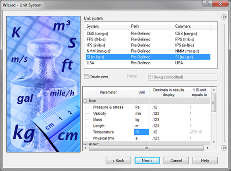
I’ll set my unit system as SI (m-kg-s) and change the unit for
temperature to °C.
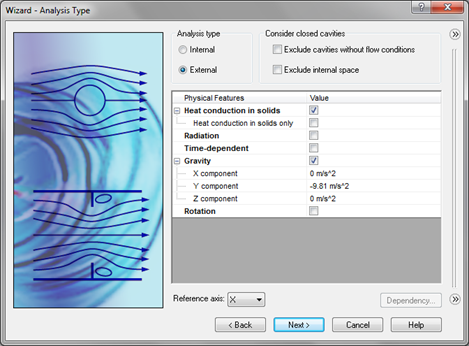
The analysis type is External because we want to consider the air
surrounding the model. I’ll turn on Heat conduction in solids and
Gravity, and confirm that Y component -9.81 m/s^2 is the correct
direction and value for this analysis.
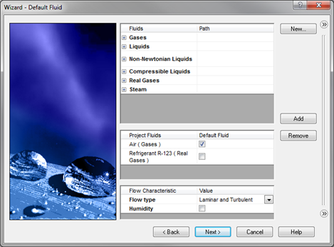
Air (Gases) and Refrigerant R-123 (Real Gases) are pre-defined
and can be added as the project fluids. I’ll make sure that the checkboxes are
set so that Air (Gases) is the Default Fluid.
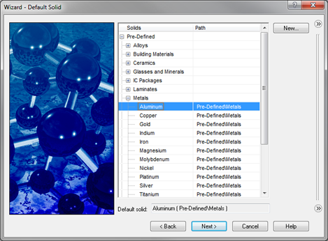
Aluminum is pre-defined under Metals and can be set as the
default solid.
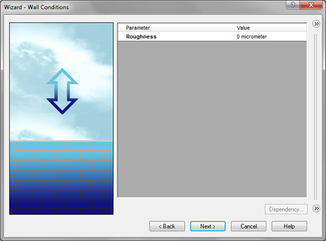
I can accept the default value of 0 micrometer for Roughness and
assume smooth walls.
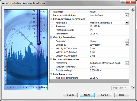
And I’ll accept the default values for the initial conditions.
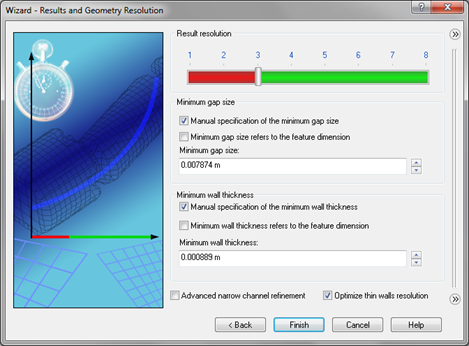
I’ll keep the Result resolution relatively low to start with and set it
to 3, and I’ll enter 0.007874 m for the
Minimum gap size and 0.000889 m for the
Minimum wall thickness, which correspond to the inner diameter and
thickness of the tube. I’ll click Finish and work my way down the Flow
Simulation analysis tree.
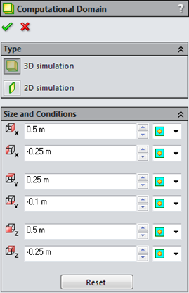
The automatically generated computational domain is bit larger than I need so
I’ll right-click Computational Domain, select Edit Definition,
and enter the following values.
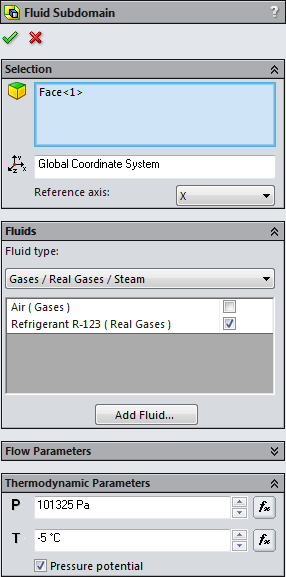
A fluid subdomain needs to be defined to set the fluid inside the tube as the
refrigerant. I’ll right-click Fluid Subdomains and select
Insert Fluid Subdomain. I’ll select an internal face of the tube, set
the checkbox next to Refrigerant R-123 (Real Gases), and enter
101325 Pa and -5 °C for the Thermodynamic Parameters.
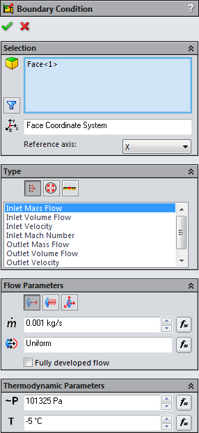
Next up are the boundary conditions. I’ll right-click
Boundary Conditions and select Insert Boundary Condition. I’ll
select the inner face of the inlet lid and define an
Inlet Mass Flow with the parameters shown below.
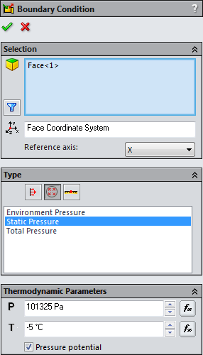
And I’ll insert another boundary condition on the inner face of the outlet lid
and define a Static Pressure as shown below.
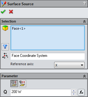
A surface source can be used to generate heat at the top of the plate. From
the Flow Simulation menu, I’ll select Insert, Surface Source.
I’ll select the top surface of the plate and enter a
Heat Generation Rate of 200 W.
The last thing to do before running the project is to define the goals. I’ll
right-click Goals, select Insert Global Goals, and select the
Max checkboxes for the Temperature (Fluid) and
Temperature (Solid).
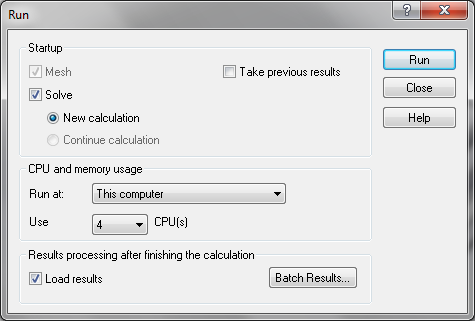
And that’s it. The project is ready to run. I’ll right-click the project name,
select Run, ensure that the checkbox for Solve is selected, and
click the Run button. This initial setup is a good start for this
problem, but it’s of course a great idea to refine the setup after running the
analysis and taking a look at the results.
Once the analysis is complete, there are many ways to investigate the results.
As an example, I’ll create a cut plot to view the temperature of the coolant
in the tube. I’ll right-click Cut Plots and select Insert. I’ll
set my plot halfway through the tube, 0.0275 m above the
Top Plane, and choose to show Temperature Contours.

The plot shows that the coolant rises from its initial temperature of -5 °C to
a maximum of about 80 °C by the end of the tube.
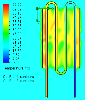
Better performance, especially at the left half of the cold plate, could
likely be achieved by reducing the temperature increase of the coolant, so
increasing the flow rate through the tube might be a good idea.
SOLIDWORKS Flow Simulation allows for changes to the design and analysis to be
cycled through at the same time and it shouldn’t be too long before an
improved cold plate is nailed down.
I hope you found this conjugate heat transfer example useful. If you have any
questions, please leave a comment and let us know.